if(!require(tibble)){install.packages("tibble");require(tibble);}
if(!require(dplyr)){install.packages("dplyr");require(dplyr);}
if(!require(readr)){install.packages("readr");require(readr);}25 25. dplyr - getting and viewing the data
The dplyr R package is part of the tidyverse family of packages. It is used to “slice and dice” tibbles to get exactly the data you want, in the form that you want it.
The dplyr R package performs the same kinds of tasks that the “SQL select statement” performs. We’ll learn more about SQL later.
Sources for info about the dplyr package:
The book “R for Data Science, second edition” is available online and in print.
The online version is here: https://r4ds.hadley.nz/ (you might need to click on the drop the small drop down menus at the top right and left of the page)*.
The intro to dplyr appears here: https://r4ds.hadley.nz/data-transformThe official tidyverse website,https://www.tidyverse.org/, is a great place to start when you’re looking for information about any of the tidyverse packages. The dplyr webpage is https://dplyr.tidyverse.org/
You can also look at the official CRAN page for dplyr, https://cloud.r-project.org/web/packages/dplyr/index.html See the vignettes on this page for good tutorial material.
25.1 Get the data
The data we are using in this section contains information about salespeople who are employees of a company. Each row of the data contains info about one salesperson. The salespeople get paid some “base pay” as well as a commission that is a percent of the total dollar amount of sales they make.
25.1.1 Load the R packages we’ll neeed
25.1.2 Download the file
The data is contained in a csv file. If you’d like to follow along with this tutorial on your own computer you can download the .csv file we are using by clicking here
25.1.3 dplyr is best used with tibbles
The majority of the dplyr functions work with tibbles or dataframes. However, the tidyverse in general and dplyr specifically is designed to work better with tibbles.
If you need to, you can always convert a tibble to a dataframe or a dataframe to a tibble.
25.1.4 Import the data by clicking on some buttons …
The code in the next section below uses read_csv function to read the data into R. If you are not comfortable with R, I recommend that you instead, follow the instructions starting in the next bullet to import the data into R.
If you are not familiar with R, you may have some trouble running the read_csv() code shown below. Instead, I recommend that you follow the following instructions to import the file into R.
To do so, click on “Import Dataset” button on the “Environment” tab (usually found in the upper-right-hand window pane in RStudio).
Choose “From Text (base)” and locate your file. You should see something like this:
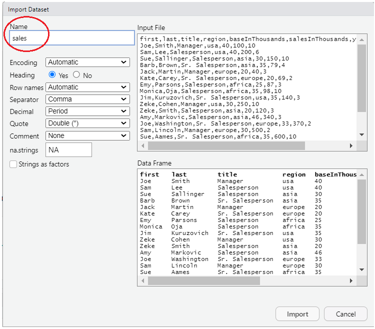
Make sure to change the “Name” portion (see circled section in picture) to read “sales”, then press the “import” button. This will open up a new tab in RStudio that shows the contents of the file. You can safely navigate away from this tab or close the tab and the data will remain imported and can be seen by typing “sales” (without the “quotes”).
Finally, in order to ensure that you are working with a tibble and not with a data.frame you can run the following R code:
sales = as_tibble(sales)
25.1.5 Import the data by typing some R code …
The following code reads the data into R. Alternatively, you can follow the instructions above to click on some buttons to import the data.
# Read in the data into a tibble
#
# Note that the following code uses the readr::read_csv function from the readr
# package which is part of the tidyverse collection of packages.
# This function is similar to the base-R read.csv function.
#
# read_csv returns a tibble, which is the data structure that the
# tidyverse packages use in lieu of dataframes. A tibble is basically
# a dataframe with extra features.
# By contrast, the base-r read.csv function returns a dataframe.

sales = read_csv("salespeople-v002.csv", na=c("","NULL"), show_col_types=FALSE)
25.2 Display the data
Since the data is in a tibble, by default, only the first 10 rows are displayed. In addition, only the columns that fit on the screen will be displayed. If the rows are too wide for the screen, then some columns may not be displayed and/or the contents of some columns may be shortened.
# Display the first few rows and columns of the sales data
sales
# A tibble: 24 × 7
first last title region baseInThousands salesInThousands yearsWithCompany
<chr> <chr> <chr> <chr> <dbl> <dbl> <dbl>
1 Joe Smith Mana… usa 40 100 10
2 Sam Lee Sale… usa 40 200 6
3 Sue Sallin… Sale… asia 30 150 10
4 Barb Brown Sr. … asia 35 79 4
5 Jack Martin Mana… europe 20 40 3
6 Kate Carey Sr. … europe 20 69 2
7 Emy Parsons Sale… africa 25 87 3
8 Monica Oja Sale… africa 35 98 10
9 Jim Kuruzo… Sr. … usa 35 140 3
10 Zeke Cohen Mana… usa 30 250 10
# ℹ 14 more rows25.3 Display more rows/columns of the tibble
25.3.1 print( SOME_TIBBLE, n=NUMBER_OF_ROWS)
# Use the print function to modify the output. Use the following arguments:
#    n - number of rows to display (Inf, i.e. infinity, for all rows)
#    width - maximum width of a row to display (might wrap if it's too long for your screen)
print(sales, n=3)
# A tibble: 24 × 7
first last title region baseInThousands salesInThousands yearsWithCompany
<chr> <chr> <chr> <chr> <dbl> <dbl> <dbl>
1 Joe Smith Mana… usa 40 100 10
2 Sam Lee Sale… usa 40 200 6
3 Sue Sallinger Sale… asia 30 150 10
# ℹ 21 more rows25.3.2 print( SOME_TIBBLE, width=WIDTH_OF_DATA)
# Display all rows and all columns
print(sales, n=Inf, width=Inf)
# A tibble: 24 × 7
first last title region baseInThousands salesInThousands
<chr> <chr> <chr> <chr> <dbl> <dbl>
1 Joe Smith Manager usa 40 100
2 Sam Lee Salesperson usa 40 200
3 Sue Sallinger Salesperson asia 30 150
4 Barb Brown Sr. Salesperson asia 35 79
5 Jack Martin Manager europe 20 40
6 Kate Carey Sr. Salesperson europe 20 69
7 Emy Parsons Salesperson africa 25 87
8 Monica Oja Salesperson africa 35 98
9 Jim Kuruzovich Sr. Salesperson usa 35 140
10 Zeke Cohen Manager usa 30 250
11 Zeke Smith Salesperson asia 20 120
12 Amy Markovic Salesperson asia 46 340
13 Joe Washington Sr. Salesperson europe 33 370
14 Sam Lincoln Manager europe 30 500
15 Sue Aames Sr. Salesperson africa 35 600
16 Barb Aames Salesperson usa 21 255
17 Jack Aames Salesperson usa 43 105
18 Kate Zeitchik Sr. Salesperson usa 50 187
19 Emy Zeitchik Manager asia 34 166
20 Monica Zeitchik Salesperson asia 23 184
21 Jim Brown Salesperson europe 50 167
22 Larry Green Sr. Salesperson europe 20 113
23 Laura White Manager africa 20 281
24 Hugh Black Sr. Salesperson africa 40 261
yearsWithCompany
<dbl>
1 10
2 6
3 10
4 4
5 3
6 2
7 3
8 10
9 3
10 10
11 3
12 3
13 2
14 2
15 10
16 7
17 4
18 4
19 4
20 1
21 2
22 4
23 8
24 925.3.3 print doesn’t change the tibble
The print function doesn’t change the tibble. print just controls what is displayed to the screen. Therefore if you save the results to a variable, the variable will still contain the entire tibble.
# display first 3 rows
print(sales, n=3)
# A tibble: 24 × 7
first last title region baseInThousands salesInThousands yearsWithCompany
<chr> <chr> <chr> <chr> <dbl> <dbl> <dbl>
1 Joe Smith Mana… usa 40 100 10
2 Sam Lee Sale… usa 40 200 6
3 Sue Sallinger Sale… asia 30 150 10
# ℹ 21 more rows# capture in a variable
x = print(sales, n=3)# A tibble: 24 × 7
first last title region baseInThousands salesInThousands yearsWithCompany
<chr> <chr> <chr> <chr> <dbl> <dbl> <dbl>
1 Joe Smith Mana… usa 40 100 10
2 Sam Lee Sale… usa 40 200 6
3 Sue Sallinger Sale… asia 30 150 10
# ℹ 21 more rows# x still contains ALL the rows
x# A tibble: 24 × 7
first last title region baseInThousands salesInThousands yearsWithCompany
<chr> <chr> <chr> <chr> <dbl> <dbl> <dbl>
1 Joe Smith Mana… usa 40 100 10
2 Sam Lee Sale… usa 40 200 6
3 Sue Sallin… Sale… asia 30 150 10
4 Barb Brown Sr. … asia 35 79 4
5 Jack Martin Mana… europe 20 40 3
6 Kate Carey Sr. … europe 20 69 2
7 Emy Parsons Sale… africa 25 87 3
8 Monica Oja Sale… africa 35 98 10
9 Jim Kuruzo… Sr. … usa 35 140 3
10 Zeke Cohen Mana… usa 30 250 10
# ℹ 14 more rows25.4 Convert between tibbles and dataframes
The majority of the dplyr functions work with tibbles or dataframes. However, the tidyverse in general and dplyr specifically is designed to work better with tibbles.
If you need to, you can always convert a tibble to a dataframe or a dataframe to a tibble.
# Convert the tibble to a data.frame
dfSales = as.data.frame(sales)

# Convert a dataframe to a tibble
tblSales = as_tibble(dfSales)

# A tibble is also a dataframe.
# This is similar to how a square is also a rectangle.
# You can see that from the class of the variable.
# The class of a tibble contains "tbl_df" "tbl" as well as "data.frame"
class(tblSales)
[1] "tbl_df" "tbl" "data.frame"# However, a dataframe is not necessarily a tibble.
# This is similar ot how a rectangle is not necessarily a square.
# Notice how the class of dfSales is only "data.frame"
class(dfSales)[1] "data.frame"# The head function is designed to work with dataframes
head(dfSales, 3) first last title region baseInThousands salesInThousands
1 Joe Smith Manager usa 40 100
2 Sam Lee Salesperson usa 40 200
3 Sue Sallinger Salesperson asia 30 150
yearsWithCompany
1 10
2 6
3 10# Therefore the head function also works with tibbles
head(tblSales, 3)# A tibble: 3 × 7
first last title region baseInThousands salesInThousands yearsWithCompany
<chr> <chr> <chr> <chr> <dbl> <dbl> <dbl>
1 Joe Smith Mana… usa 40 100 10
2 Sam Lee Sale… usa 40 200 6
3 Sue Sallinger Sale… asia 30 150 10#######################################################################
# However, features of some functions that are designed to
# work with tibbles might not work with data.frames.
######################################################################## This works fine - display the first 3 rows of the tibble.
print(tblSales, n=3) # A tibble: 24 × 7
first last title region baseInThousands salesInThousands yearsWithCompany
<chr> <chr> <chr> <chr> <dbl> <dbl> <dbl>
1 Joe Smith Mana… usa 40 100 10
2 Sam Lee Sale… usa 40 200 6
3 Sue Sallinger Sale… asia 30 150 10
# ℹ 21 more rows# ERROR - n argument is not designed to work with dataframes that aren't tibbles
print(dfSales, n=3) Error in print.default(m, ..., quote = quote, right = right, max = max): invalid 'na.print' specification25.5 getting “slices” of the rows
Among some of the many functions included in dplyr are the various “slice_…” functions. These functions return a new tibble with just the specified rows. The new tibble can be saved in a variable. This is different from how the print function works (see above).
The functions can take several arguments that modify their behavior. The following are just a few examples. See the ?slice for more info about these functions and their arguments.
25.5.1 slice_sample()
slice_sample() chooses a random sample of the rows.
# see 3 randomly chosen rows
sales |> slice_sample(n=3)
# A tibble: 3 × 7
first last title region baseInThousands salesInThousands yearsWithCompany
<chr> <chr> <chr> <chr> <dbl> <dbl> <dbl>
1 Barb Brown Sr. … asia 35 79 4
2 Monica Zeitchik Sale… asia 23 184 1
3 Sue Salling… Sale… asia 30 150 10# randomly chose 10% of the rows to view
sales |> slice_sample(prop=0.10) # A tibble: 2 × 7
first last title region baseInThousands salesInThousands yearsWithCompany
<chr> <chr> <chr> <chr> <dbl> <dbl> <dbl>
1 Sue Sallinger Sale… asia 30 150 10
2 Jack Aames Sale… usa 43 105 425.5.2 slice_min() and slice_max()
To see the rows that correspond to the min or max values of a specified column use slice_min()/slice_max().
# see rows with 3 smallest salesInThousands
sales |> slice_min(order_by=salesInThousands, n=3)
# A tibble: 3 × 7
first last title region baseInThousands salesInThousands yearsWithCompany
<chr> <chr> <chr> <chr> <dbl> <dbl> <dbl>
1 Jack Martin Manager europe 20 40 3
2 Kate Carey Sr. Sal… europe 20 69 2
3 Barb Brown Sr. Sal… asia 35 79 4# see rows with 3 smallest salesInThousands
sales |> slice_max(order_by=salesInThousands, n=3) # A tibble: 3 × 7
first last title region baseInThousands salesInThousands yearsWithCompany
<chr> <chr> <chr> <chr> <dbl> <dbl> <dbl>
1 Sue Aames Sr. … africa 35 600 10
2 Sam Lincoln Mana… europe 30 500 2
3 Joe Washingt… Sr. … europe 33 370 225.5.3 slice() to see specific rows
You don’t need c() to specify the rows. This is typical of the style of functions in the tidyverse.
# get rows 1,5,7 in a new dataframe
x |> slice(1,5,7)
# A tibble: 3 × 7
first last title region baseInThousands salesInThousands yearsWithCompany
<chr> <chr> <chr> <chr> <dbl> <dbl> <dbl>
1 Joe Smith Manager usa 40 100 10
2 Jack Martin Manager europe 20 40 3
3 Emy Parsons Salesp… africa 25 87 3# get all rows except for rows 5 through 22
x |> slice(-(5:22))# A tibble: 6 × 7
first last title region baseInThousands salesInThousands yearsWithCompany
<chr> <chr> <chr> <chr> <dbl> <dbl> <dbl>
1 Joe Smith Mana… usa 40 100 10
2 Sam Lee Sale… usa 40 200 6
3 Sue Sallinger Sale… asia 30 150 10
4 Barb Brown Sr. … asia 35 79 4
5 Laura White Mana… africa 20 281 8
6 Hugh Black Sr. … africa 40 261 925.5.4 slice_head() and slice_tail()
The slice_head() and slice_tail() are very similar to the base-R head() and tail() functions. They return the first few (slice_head) or last few (slice_tail) rows from a tibble.
# get just first 3 rows
sales |> slice_head(n=3)
# A tibble: 3 × 7
first last title region baseInThousands salesInThousands yearsWithCompany
<chr> <chr> <chr> <chr> <dbl> <dbl> <dbl>
1 Joe Smith Mana… usa 40 100 10
2 Sam Lee Sale… usa 40 200 6
3 Sue Sallinger Sale… asia 30 150 10print(n=3) vs slice_head(3)
# get just first 3 rows
sales |> slice_head(n=3)
# A tibble: 3 × 7
first last title region baseInThousands salesInThousands yearsWithCompany
<chr> <chr> <chr> <chr> <dbl> <dbl> <dbl>
1 Joe Smith Mana… usa 40 100 10
2 Sam Lee Sale… usa 40 200 6
3 Sue Sallinger Sale… asia 30 150 10# save that in a variable
x = sales |> slice_head(n=3)
# x only contains 3 rows
x# A tibble: 3 × 7
first last title region baseInThousands salesInThousands yearsWithCompany
<chr> <chr> <chr> <chr> <dbl> <dbl> <dbl>
1 Joe Smith Mana… usa 40 100 10
2 Sam Lee Sale… usa 40 200 6
3 Sue Sallinger Sale… asia 30 150 10# print appears to do the same thing
# but print only affects what is displayed to the screen, not
# what is "returned" and can be saved in a variable.
y = sales |> print(n=3)# A tibble: 24 × 7
first last title region baseInThousands salesInThousands yearsWithCompany
<chr> <chr> <chr> <chr> <dbl> <dbl> <dbl>
1 Joe Smith Mana… usa 40 100 10
2 Sam Lee Sale… usa 40 200 6
3 Sue Sallinger Sale… asia 30 150 10
# ℹ 21 more rows# y still has all of the rows
y# A tibble: 24 × 7
first last title region baseInThousands salesInThousands yearsWithCompany
<chr> <chr> <chr> <chr> <dbl> <dbl> <dbl>
1 Joe Smith Mana… usa 40 100 10
2 Sam Lee Sale… usa 40 200 6
3 Sue Sallin… Sale… asia 30 150 10
4 Barb Brown Sr. … asia 35 79 4
5 Jack Martin Mana… europe 20 40 3
6 Kate Carey Sr. … europe 20 69 2
7 Emy Parsons Sale… africa 25 87 3
8 Monica Oja Sale… africa 35 98 10
9 Jim Kuruzo… Sr. … usa 35 140 3
10 Zeke Cohen Mana… usa 30 250 10
# ℹ 14 more rowsbase-R head() vs dplyr::slice_head()
When used alone, slice_head() and head() are very similar.
However, slice_head() and slice_tail(), as well as the other slice_* functions are designed to work well in conjunction with the dplyr::group_by() function (we will cover group_by() later). The head() and tail() functions are not.
The general rule is that if you are using several dplyr functions in a pipeline (i.e. %>%> or |>) you should opt for the dplyr functions instead of the base-R functions that might seem similar.
25.6 Other ways of viewing the data
# To see the entire tibble in a separate tab in RStudio
# you can use the following command
#
#View(sales)

# Show all column names and datatypes plus some actual data
glimpse(sales)

# Show just the column names (could be useful for a quick reminder when you need it)
colnames(sales)